Improving MPPI for High-Inertia Industrial Vehicles
If you’ve ever tried to navigate a 4-ton warehouse robot, you know that “move carefully” is not just a suggestion: it’s a physics problem. Heavy industrial vehicles with raised centers of gravity, like Dexory’s autonomous inventory scanning towers, cannot accelerate or decelerate the way a lightweight AMR can. Commanding even modest jerks can tip product, stress mechanical joints, or simply cause the drivetrain to fight the controller. Yet until now, Nav2’s MPPI controller was tuned for the nimble end of the spectrum, with default acceleration limits of 3.0 m/s^2, more than ten times what some industrial platforms can safely handle.
This post walks through the investigation and set of fixes we developed to make MPPI reliably respect low and asymmetric acceleration constraints. The work was motivated by Dexory, whose tall scanning towers require acceleration limits as low as 0.25 m/s^2 forward and -0.5 m/s^2 braking which is an order of magnitude below the defaults typically used. The result is a set of carefully validated improvements that benefit not just Dexory, but every team pushing Nav2 onto heavier, higher-inertia platforms.
We write these musings up as a blog post because it is a nice, confined challenge to solve in a highly technical part of the Nav2 project. Hopefully this provides useful context and learnings for future engineers about both MPPI itself and understanding these changes in detail.
The Core Problem: cvx vs vx in MPPI
MPPI (Model Predictive Path Integral) control works by sampling thousands of candidate trajectories, scoring them, and blending the best ones into a smooth control output. Internally, the optimizer distinguishes between control velocities (cvx, the raw control efforts) and state velocities (vx, what the robot would actually do after applying the controls considering the physical limits and reactions).
Originally, MPPI updated the controls cvx used in the optimization during the motion model projection to match the state velocities vx. This is done as the controls are what should be sent to the vehicle in order to result in the intended state velocity. However, the controls are supposed to be raw and not adjusted by the prediction of next states or its dynamic limits such that the controls yeild the velocities. Thus, PR #5266 implemented an analogous change for acceleration handling, so the controls would not be clamped by acceleration limits, only the state velocities used for trajetory rollouts:
- state.cvx.col(i - 1) = state.cvx.col(i - 1)
-   .cwiseMax(lower_bound_vx)
-   .cwiseMin(upper_bound_vx);
- state.vx.col(i) = state.cvx.col(i - 1);
+ state.vx.col(i) = state.cvx.col(i - 1)
+   .cwiseMax(lower_bound_vx)
+   .cwiseMin(upper_bound_vx);
We believe this is technically correct. The motion model is supposed to model the robot’s actual capabilities. You send a cvx and you get a vx out, so vx is used for trajectory rollouts of what the vehicle actually does for scoring, while cvx is used in the optimization softmax. When setting acceleration limits artificially low in the motion model, there needs to be a complementary system between the controller and the base hardware to enact that limit (the velocity smoother or base controller) such that the system acts the way the motion model predicted.
However (funnily enough), this broke acceleration limitation behavior even further. More discussion followed in Issue #5464 and Issue #5214, where users reported two main problems:
- Acceleration limits were not being fully respected in the output commands
- Increased oscillation / wobble in the angular velocity at steady state
A user noted that switching to open-loop odometry made the wobble go away on their robot with execution latency and low acceleration limits. Steve believes what’s happening is that the odometry from executing noisy controls causes the noise effects to be amplified. So this is really a band-aid solution.
We set out to understand both issues from first principles, fix them properly, and validate each change with data.
Investigation 1: Unclamped Controls and Angular Response
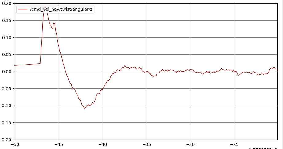
We created a controlled test by sending a straight-line path offset 0.5 m laterally from the robot and driving 8m forward, using the low-acceleration asymmetric limits (0.25 m/s^2 forward, -0.5 m/s^2 braking, 1.2 rad/s^2 angular). We generated the path via CLI to remove any variabilities due to path planning.
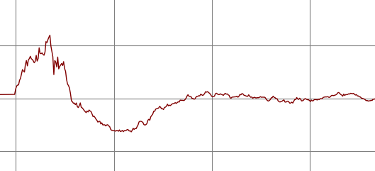
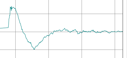
Angular velocity response, before unclamping (left) and after (right):
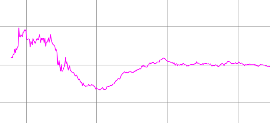
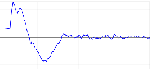
Top: clamped controls. Bottom: unclamped (raw) controls used in optimization.
Each grid box is 0.2 rad/s. The unclamped version shows a wider initial correction and slightly more noise at steady state, but converges onto the path faster due to the sharper response (possibly out of dynamic limits).
With standard (high) acceleration limits, the difference is minimal. Just a touch more noise at steady state:
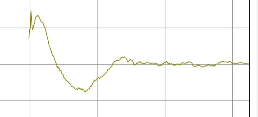
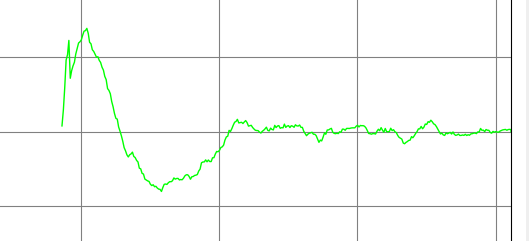
Top: clamped controls, full acceleration. Bottom: unclamped controls, full acceleration.
Using open-loop odometry with low-acceleration limits, we again see the higher maximum velocities (possibly more noise between the two?) but consistent convergence times. The noise compared to the original unclamped closed-loop is certainly improved, so we can see why users thought open-loop would be a viable short-term solution:
Left: clamped, open-loop. Right: unclamped, open-loop.
So far so good; just more noise in tracking which we expected.
Investigation 2: Are Acceleration Limits Actually Respected?
Now, we were curious: what accelerations are actually being used, because they seem higher? The sharpness of the dip and adjustment back onto the path implies less lag/smoothing occurring, which would make sense if we’re using unbounded controls for the optimization rather than the bounded velocities. However we were concerned that the acceleration limits weren’t being respected.
First, we verified that intra-trajectory constraints are enforced. We added a check at the end of optimize() that computes the acceleration between each pair of consecutive optimal control samples and warns if any violate the configured limits:
const int n = control_sequence_.vx.size();
if (n > 1) {
  const float dt = settings_.model_dt;
  Eigen::ArrayXf ax = (control_sequence_.vx.tail(n-1) -
    control_sequence_.vx.head(n-1)) / dt;
  Eigen::ArrayXf az = (control_sequence_.wz.tail(n-1) -
    control_sequence_.wz.head(n-1)) / dt;
  // ... check ax/az against constraints, warn on violation
}
Minor a very minor edge case that rarely triggers (which we fixed), this worked as intended. Checkmark: acceleration constraints within the optimal control sequence are being respected.
The other source of potential violations is the initialization of candidate velocities at the robot’s odometric speed. In closed-loop mode, odometry seeds the velocities; in open-loop, the last control’s commanded velocity is used instead (assuming perfect execution to handle odometry lag/noise).
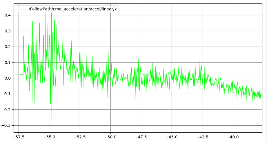
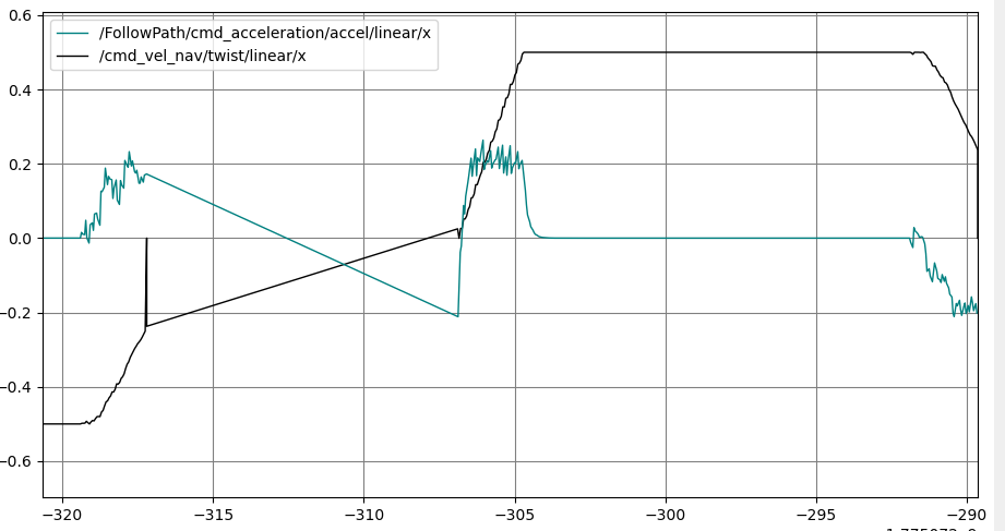
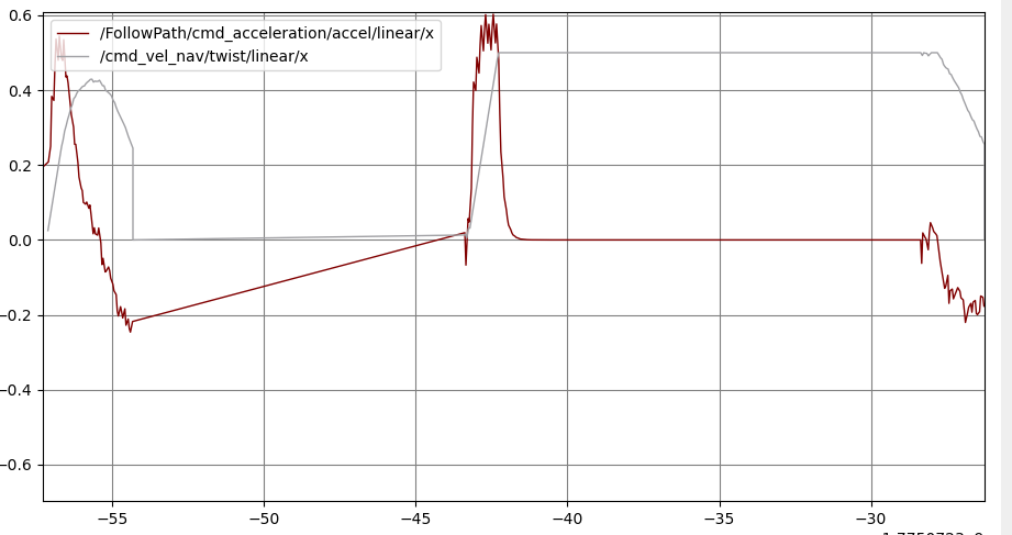
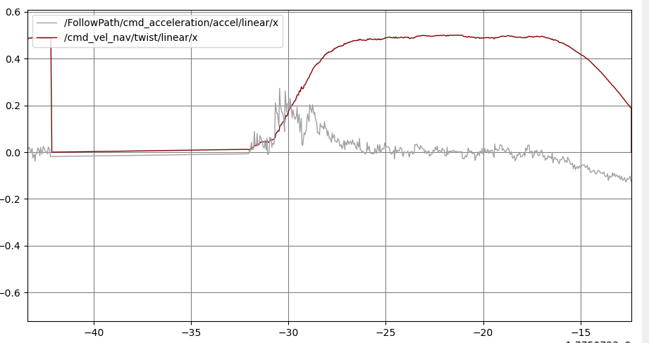
We instrumented the controller to publish the actual commanded accelerations:
accel_msg.accel.linear.x =
  (control.twist.linear.x - last_command_vel_.linear.x) / controller_period_;
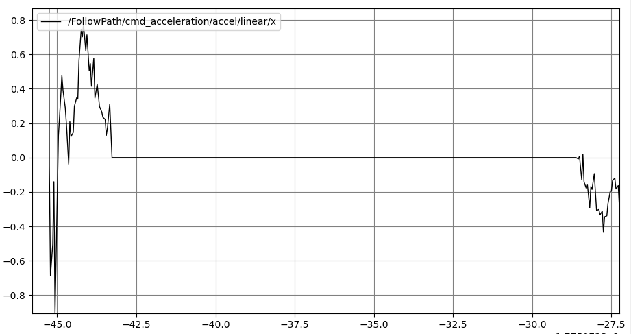
Clamped controls: acceleration stays roughly within bounds but with extreme chattering:
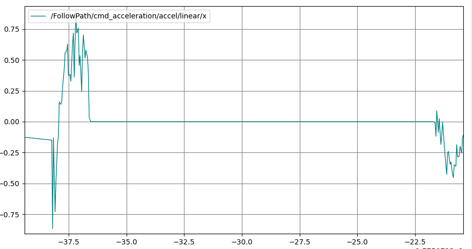
Unclamped controls: much smoother acceleration profile, but the limits are violated during the initial ramp-up (note the y-axis scale difference!):
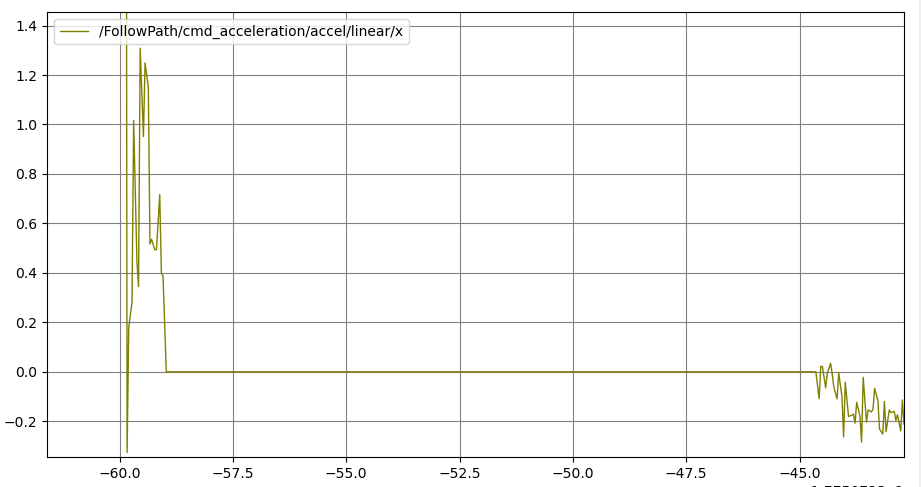
This is genuinely interesting. The smoothness improvement with unclamped controls is significant. We believe intuitively that the additional velocity noise in the clamped case is because the softmax is scoring trajectory points based on clamped values, so it can’t see “how bad” a violation is (scoring bad trajectories worse leads to less use in the final output). Meanwhile the jitter in the clamped version comes from the optimization being unable to distinguish “slightly over the limit” from “massively over”.
But regardless, the constraint violations in the unclamped case needed to be fixed.
The model_dt vs control_period Mismatch
One important clue: the controller_period runs at 20 Hz (0.05s) but the model_dt used in the optimizer is 0.1s. The acceleration limits are applied within the trajectory optimization using model_dt. That means the acceleration constraints in the optimizer are simulated at twice the duration of what the controller actually grabs to execute, virtually doubling the acceleration limits of cmd_vel output. When we make them the same:
And with open-loop, virtually the same thing with no meaningful differentiation:
We’re still regularly violating the acceleration constraints externally, even with matched timing and open-loop. Clearly its not an issue solely with configuration nor is it an issue with the internal dynamic limits.
Root Cause: Inter-Iteration Feasibility
It became clear at this point what was happening. The intra-trajectory dynamic limits are correctly set, but when we have a speed as the initial state, that is never being checked against the validity of the first optimal control sample. The optimal control sequence has the speed set as current vx(0) = speed.x to initialize, but that is not being done in the controls which are used to compute/override the optimal trajectory at the end of the process. Now that the cvx are unbounded by the acceleration limits, the first control is even more free to do anything it wishes, though even when it was bounded it could still cause these issues.
The Fix: Two-Part Acceleration Feasibility
-
Hard guardrails in
applyControlSequenceConstraints(): Add acceleration constraints relative to the starting speed to ensure the trajectory is feasible to execute from the current state as well as within the optimal trajectory. These are the hard “we know we’re going to be feasible” guardrails. -
Soft initialization of
cvx.col(0): Add the initial acceleration constraint to the first samples in the optimal control sequence before noising it for generating controls, with respect to the current speed. Rather than simply setting it to the initial speed, we clamp the control sequence by the acceleration limits so we don’t modify it unless we absolutely have to. This keeps the trajectory shape realistic during scoring rather than waiting for the end to clamp inapplyControlSequenceConstraintsand deforming the shape without a chance to score with that in mind.
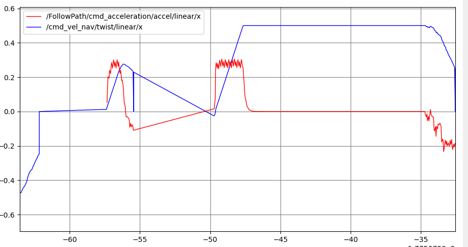
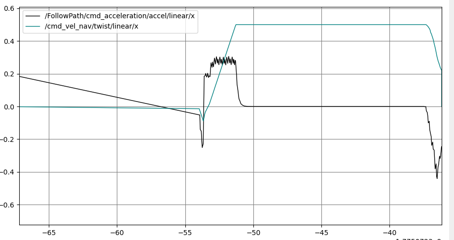
The results were immediate. We tested all four configurations:
Closed-loop, model_dt equal to control frequency:
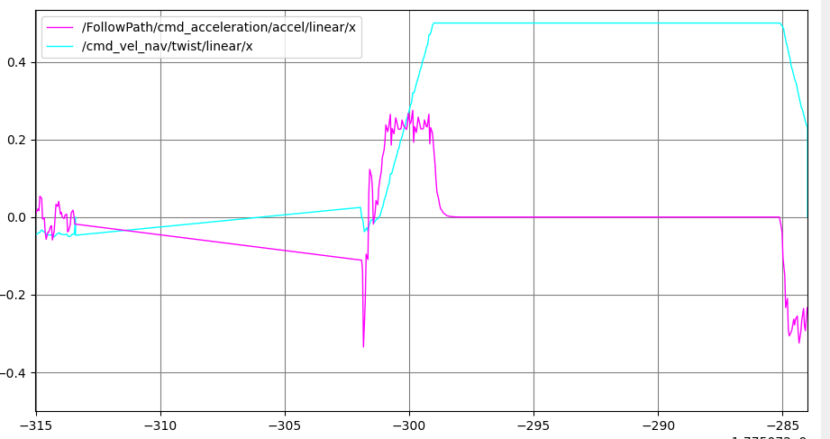
Acceleration (magenta) now stays within bounds while velocity (cyan) ramps smoothly.
Open-loop, model_dt equal to control frequency:
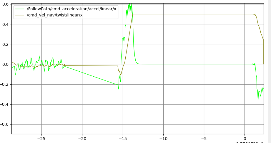
Closed-loop, model_dt not equal to control frequency:
Open-loop, model_dt not equal to control frequency:
For closed-loop configurations, the acceleration constraints are respected and we ramp up to the velocity with feedback so it takes a bit longer. For open-loop configurations, we still interestingly violate the constraint. This seems due to the fact that we do the t=0 acceleration constraint using model_dt rather than the actual control_frequency. Since we don’t have real odometry to ground us into reality in open-loop, it uses the acceleration corresponding to accel * model_dt / control_frequency (in this case: x2) when they are not the same. Using the control_period instead during the acceleration constraint in (1) and (2) above fixes this case:
However, when model_dt equals the control frequency, we still saw violations. This took several hours to figure out. Essentially the shifting logic “skips” the first control sample vx(0) and applies vx(1). It’s pretty obvious we then allow ourselves to use an additional timestep which lets us double the acceleration limits, precisely.
How to fix this cleanly up-front (and not in post-processing) took some pencil and paper work. The solution is where we apply the acceleration constraints based on speed, we need to hard-set the t=0 index to be the speed, such that t=1 is required to be within dynamic limits of that current speed by 1 timestep duration. This only applies for the case of model_dt = control_frequency. Otherwise, we let it float as any value as long as it is within the acceleration limit window.
Viola!
So Steve: Do We Still Need Unclamped Controls After All?
With all the feasibility fixes in place, we sanity-checked whether clamping the controls again would be acceptable. The answer: Uhhhh yeah, we really do need unclamped controls.
Re-clamping the controls reintroduces chattering and poor acceleration tracking despite all other fixes.
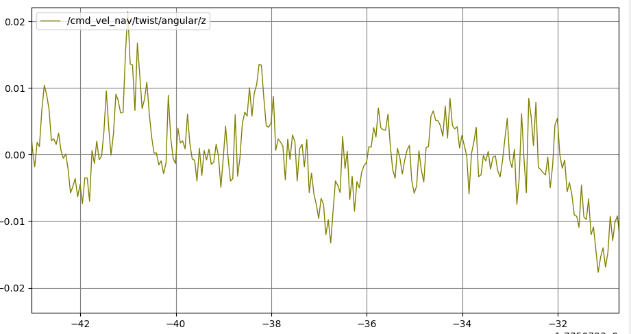
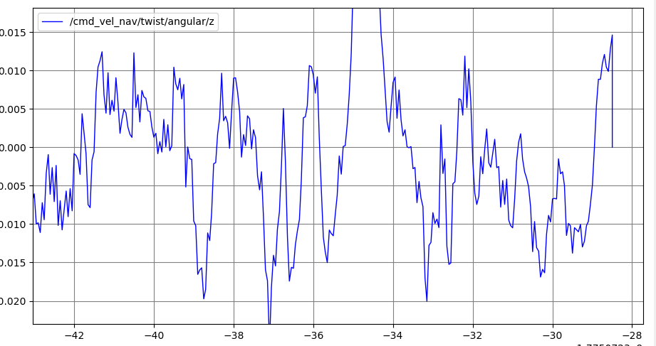
Investigation 3: Characterizing & Improving the Oscillation / Wobble
With acceleration limits properly enforced, we turned to the second reported issue: increased angular velocity noise at steady state. We need to characterize the noise before we can evaluate solutions.
We updated the test to drive 12 m instead of 8 m to increase the steady-state data we inspect. Plotting the angular velocity after the robot converges onto the path:
Before (clamped controls): General noise in +/- 0.02 rad/s, with spikes up to +/- 0.04 rad/s. Best-case noise across multiple runs was around 0.01 rad/s.
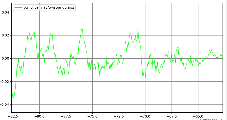
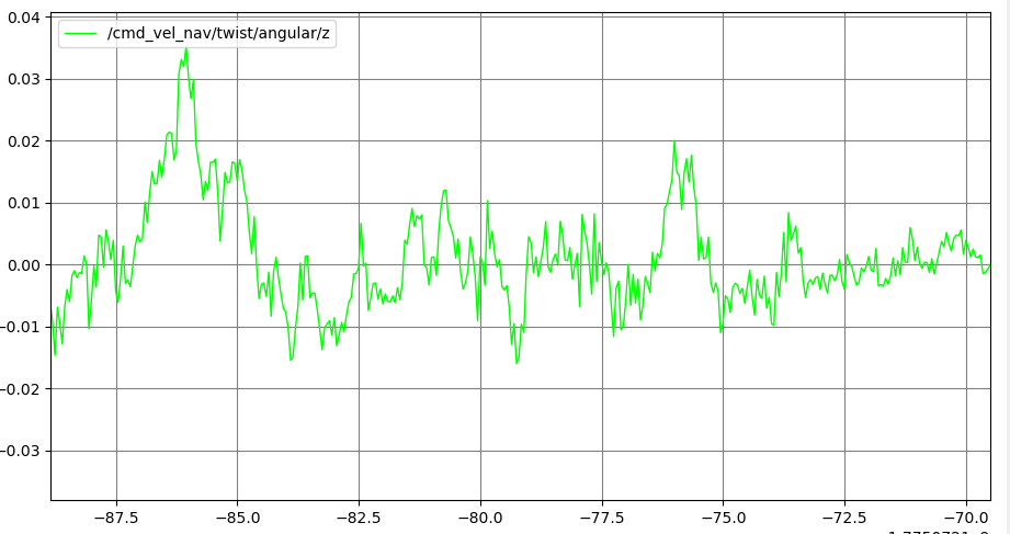
After (unclamped controls): General noise in +/- 0.02 rad/s with similar spikes. Qualitatively from multiple runs, we were unable to see noise below 0.02 rad/s (vs. 0.01 rad/s best-case before), so there does seem to be some noise increase worth addressing.
We did not observe the dramatic “wobble” effect that some users reported, but that may be due to model lag in their systems. Other work adding model lag to the system may be required to reproduce that, but we can still work on improving the noise regardless.
Attempt 1: Removing Importance Sampling (gamma)
There are notes in various publications that the importance sampling term isn’t terribly important and may contribute to noise. Let’s remove it and see:
// auto bounded_noises_vx = state_.cvx.rowwise() - vx_T;
// const float gamma_vx = s.gamma / (s.sampling_std.vx * s.sampling_std.vx);
// costs_ += (gamma_vx * (bounded_noises_vx.rowwise() * vx_T)
//   .rowwise().sum()).eval();
// ... same for wz, vy
Definitely worse, noise > 0.035 rad/s. Moving on from that idea.
Attempt 2: More Aggressive Savitzky-Golay Filtering
We tried two approaches. First, applying the SGF a second time after control constraints are enforced for a double smoothing effect. This did reduce the noise a bit, but we still saw spikes on the order of 0.03 rad/s and general noise around 0.02 rad/s. While the general noise is more tightly bounded, it’s not the clear difference-maker we’re looking for, and it’s kind of hacky.
Second, we dropped the filter to 1st order so it essentially becomes a weighted mean average which should very effectively remove noise at the cost of detail. This actually did a pretty decent job:
A good option to consider, but let’s keep exploring. This doesn’t seem like the best solution.
Attempt 3: Tuning Temperature and Gamma
Increasing temperature does successfully reduce the magnitude of the noise, but may be slower to react to dynamic obstacles or changes. Additionally, the noise spikes are quite significant and change sign frequently in large swings:
We could say that this “works” but we don’t think this is what anyone would want. This basically relies on the optimization problem averaging using a larger number of samples to reduce noise. Manipulating gamma did not seem to have a great impact either, so we’ll skip that analysis.
Attempt 4: Reducing Sampling Standard Deviation (the winner)
Let’s do some back-of-the-envelope math. We’re currently using a STD of 0.2 for linear and angular velocities. That puts us within 1 sigma of 0.2 m/s and 0.2 rad/s for each timestep. If the timestep is 0.1s, then with an acceleration limit of 0.25 m/s^2, we’re only actually able to differ by a measly 0.025 m/s per step, significantly lower than our noised values. For a STD of 0.2 to make sense, we would need to be able to accelerate proportional to ~0.2 m/s (or rad/s) in a single timestep, which amounts to 2 m/s^2. That is totally sane for a normal AMR without low acceleration limits, hence why we have such a value set for Nav2 by default.
But for low-acceleration platforms, we’re exploring mostly physically unreachable states, adding noise without information.
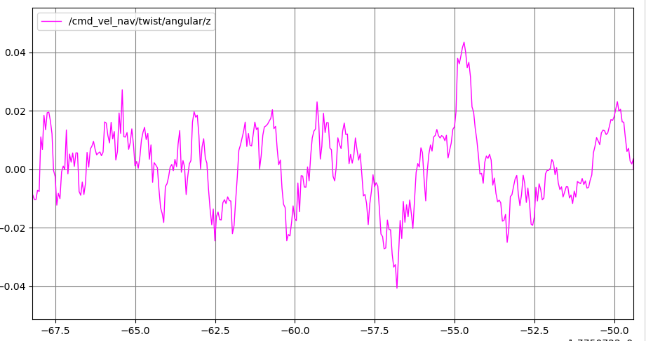
Reducing the STD to 0.1, we see a pretty big reduction in noise while still exploring far more than we can realistically achieve with the acceleration limits in place:
Full trajectory with reduced STD: clean response matching the original clamped behavior.
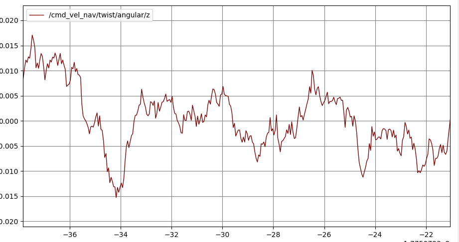
Steady-state noise well under +/- 0.01 rad/s, better than the original clamped controls.
Now that’s more like it. The complete chart looks very similar to the original before graphics and the noise distributions are well below the before graphics. Our spikes are in the +/- ~0.015 rad/s range with normal noise well under +/- 0.01 rad/s. This is also less noisy and more consistent than the SGF order 1 chart, so we would say this is a better option. However we think it is still wise to take the learnings from this experience and offer the SGF option for reducing the order if users want additional smoothing.
Reducing the STD is a complete and legitimate solution to the noise increase from using low acceleration with unclamped controls.
Investigation 4: Asymmetric Acceleration Limits
One pleasant surprise: asymmetric acceleration support (higher braking deceleration than forward acceleration) was completely resolved by the work above. The inter-iteration feasibility fixes and unclamped controls naturally handle the different forward/reverse limits through the same constraint machinery. No additional work needed. See the acceleration plots above to confirm that the asymmetric limits (0.25 m/s^2 forward, -0.5 m/s^2 braking) are being properly respected.
Summary of Changes
The complete set of improvements:
- Unclamped raw control velocities in the MPPI optimization, allowing the optimizer to freely explore the control space unclamped while the motion model enforces physical limits on state trajectories
- Inter-iteration acceleration feasibility ensuring the transition between optimization iterations respects the robot’s current dynamic state
- Proper timing alignment between
model_dtandcontrol_periodfor acceleration constraint enforcement at the trajectory boundary - Control sequence shift correction to prevent the shifting logic from granting an extra timestep of unconstrained acceleration
- Reduced sampling standard deviations proportional to what the acceleration limits actually allow, eliminating noise from sampling physically unreachable states
These changes make MPPI viable for the growing class of heavy industrial robots that need precise, low-acceleration control: warehouse towers, mining vehicles, agricultural platforms, and more. The fixes correct fundamental assumptions in the optimization that happened to be invisible at high acceleration limits but became critical at low ones.
Overall, we’ve done an excellent job improving the behavior of MPPI not just for low-acceleration cases, but in general. The acceleration profiles are dramatically smoother, the constraints are reliably enforced, and the steady-state tracking noise is actually better than before.
If you’re working with high-inertia platforms, give these changes a try and let us know how they work for you!
Our Sponsors
Platinum

Gold


Silver


Friends of Nav2


Stay Updated
Follow us for more news and updates.